在离散行为空间中,Q-learning 的策略选择与目标值为: \[ \pi(a_t|s_t)= \begin{cases} 1 & \quad \text{if } a_t=\arg\max_{a_t}Q_\phi(s_t,a_t)\\ 0 & \quad \text{otherwise} \end{cases}\\ \ \\ y_j=r_j+\gamma\max_{a_j'}Q_{\phi'}(s_j',a_j') \] 但在连续行为空间中,这两者的 \(\max\) 操作就会出现问题。
一种最简单的解决方法是: \[ \max_aQ(s,a) \approx \max\{Q(s,a_1),\cdots,Q(s,a_N)\} \] 其中 \((a_1,\cdots,a_N)\) 以某种分布进行采样得到(比如均匀分布)。这种方法尽管很方便且能并行操作,但并不十分准确,尤其是在维度增加的情况下。
第二种,来自于论文 Continuous deep q-learning with model-based acceleration
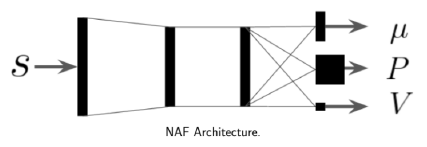
论文中,作者精心构造了由优势函数与状态价值函数组成的 \(Q\) 函数,取名为 Normalized Advantage Functions (NAF): \[ \begin{align*} Q(s,a|\theta^Q) &= A(s,a|\theta^A)+V(s|\theta^V)\\ A(s,a|\theta^A) &= -\frac{1}{2}(a-\mu(s|\theta^\mu))^T P(s|\theta^P) (a-\mu(s|\theta^\mu)) \\ P(s|\theta^P) &= L(s|\theta^P) L(s|\theta^P)^T \end{align*} \] 其中 \(L(s|\theta^P)\) 为下三角矩阵,它可以来自于神经网络的线性输出。这样构造 \(Q\) 函数的好处是,可以发现 \(A\) 函数是一个负的半正定二次型矩阵,这样一来有如下两个特点: \[ \arg\max_a Q_\theta(s,a)=\mu_\theta(s) \\ \max_a Q_\theta(s,a)=V_\theta(s) \]
整个网络的架构为:
算法如下:
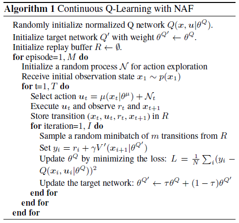
这么做的话,算法和原来的 Q-learning 一样。但是缺点就在于 \(Q\) 函数只能是固定的形式(如这里的二次函数),非常受限, \(Q\) 函数的建模泛化能力将大大降低。
论文中还提出了基于模型的使用 iLQR 方法来加速训练,此处不再说明。
第三种是使用 Deep Deterministic Policy Gradient 算法。