本文翻译自 Natural Gradient Descent, Agustinus Kristiadi.
假设我们现在有一个概率模型 \(p(x|\theta)\) ,我们希望通过最大化似然函数来找到最优的参数 \(\theta\),也就是最小化损失函数 \(\mathcal{L}(\theta)\) ,即负的似然函数。 一般用来解决优化问题的方法是使用梯度下降法,我们根据 \(-\nabla \mathcal{L}(\theta)\) 的方向来使参数向前走一步,这个方向是 \(\theta\) 在参数空间中最陡峭的方向。可以用如下公式表示: \[ \frac{-\nabla_\theta \mathcal{L}(\theta)}{\lVert \nabla_\theta \mathcal{L}(\theta) \rVert} = \lim_{\epsilon \to 0} \frac{1}{\epsilon} \mathop{\text{arg min}}_{\text{ s.t. } \lVert d \rVert \leq \epsilon} \mathcal{L}(\theta + d) \, . \] 意思就是要去选取一个向量 \(d\) ,使得新参数 \(\theta +d\) 在参数 \(\theta\) 的距离为 \(\epsilon\) 的范围内,并能最小化损失。注意我们在描述这个范围的时候用的是欧几里得范数,因此梯度下降取决于参数空间(parameter space)的欧几里得几何。
但如果我们的目标是使损失函数最小(使似然性最大化),那么很自然地,我们会在所有可能的似然性空间中让参数向前走一步。 由于似然函数本身是概率分布,因此我们可以将其称为分布空间(distribution space) 。 因此,在该分布空间而不是参数空间中采用最陡的下降方向是有意义的。
那么我们应该在该空间中使用哪个度量/距离呢?一个流行的选择是 KL 散度。
从下图可以看出在参数空间中仅使用欧几里得距离会出现问题。考虑两个高斯分布,变量只为均值,方差固定为 2 和 0.5。
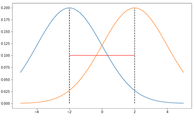
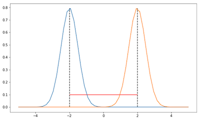
在这两张图中,两个高斯的距离是相同的,根据欧几里德距离也就是 4 (红线),但在分布空间中,也就是说我们考虑一下这两个高斯的形状,这两张图中的高斯距离是不一样的。第一幅的 KL 散度会更小一点因为两个高斯有更多的重叠。因此如果我们只考虑参数空间那么会遗漏分布之间的信息。
Fisher and KL-divergence
Fisher 信息矩阵(Fisher Information Matrix)定义了以 KL 散度为度量标准的分布空间中的局部曲率。
定理:Fisher 信息矩阵(FIM)是关于 \(\theta'\) ,在 \(\theta=\theta'\)处, 两个分布 \(p(x|\theta)\) 与 \(p(x|\theta')\) 的 KL 散度的 Hessian 矩阵。
证明:KL 散度可以拆分为熵和交叉熵两部分: \[ \text{KL} [p(x \vert \theta) \, \Vert \, p(x \vert \theta')] = \mathbb{E}_{p(x \vert \theta)} [ \log p(x \vert \theta) ] - \mathbb{E}_{p(x \vert \theta)} [ \log p(x \vert \theta') ] \, . \] 关于 \(\theta'\) 的一阶导为: \[ \begin{align} \nabla_{\theta'} \text{KL}[p(x \vert \theta) \, \Vert \, p(x \vert \theta')] &= \nabla_{\theta'} \mathbb{E}_{p(x \vert \theta)} [ \log p(x \vert \theta) ] - \nabla_{\theta'} \mathbb{E}_{p(x \vert \theta)} [ \log p(x \vert \theta') ] \\[5pt] &= - \mathbb{E}_{p(x \vert \theta)} [ \nabla_{\theta'} \log p(x \vert \theta') ] \\[5pt] &= - \int p(x \vert \theta) \nabla_{\theta'} \log p(x \vert \theta') \, \text{d}x \, . \end{align} \] 二阶导为: \[ \begin{align} \nabla_{\theta'}^2 \, \text{KL}[p(x \vert \theta) \, \Vert \, p(x \vert \theta')] &= - \int p(x \vert \theta) \, \nabla_{\theta'}^2 \log p(x \vert \theta') \, \text{d}x \\[5pt] \end{align} \] 那么关于 \(\theta'\) ,在 \(\theta=\theta'\)处的 Hessian 为: \[ \begin{align} \text{H}_{\text{KL}[p(x \vert \theta) \, \Vert \, p(x \vert \theta')]} &= - \int p(x \vert \theta) \, \left. \nabla_{\theta'}^2 \log p(x \vert \theta') \right\vert_{\theta' = \theta} \, \text{d}x \\[5pt] &= - \int p(x \vert \theta) \, \text{H}_{\log p(x \vert \theta)} \, \text{d}x \\[5pt] &= - \mathbb{E}_{p(x \vert \theta)} [\text{H}_{\log p(x \vert \theta)}] \\[5pt] &= \text{F} \, . \end{align} \]
分布空间中最速下降
现在我们已经准备好用 FIM 来加强梯度下降。但首先我们要推导一下 KL 散度在 \(\theta\) 周围的泰勒展开。
定理:令 \(d\rightarrow 0\) ,KL 散度的泰勒二阶展开式为 \(\text{KL}[p(x \vert \theta) \, \Vert \, p(x \vert \theta + d)] \approx \frac{1}{2} d^\text{T} \text{F} d.\)
证明:我们用 \(p_\theta\) 来表示 \(p(x|\theta)\) 。根据定义,函数 \(f(\theta)\) 在点 \(\theta=\theta'\) 处的泰勒二阶展开为: \[ f(\theta') \approx f(\theta) + (\theta'-\theta)^T\nabla f(\theta) + \frac{1}{2}(\theta'-\theta)^TF(\theta'-\theta) \] 那么 KL 散度的泰勒二阶展开为: \[ \begin{align} \text{KL}[p_{\theta} \, \Vert \, p_{\theta + d}] &\approx \text{KL}[p_{\theta} \, \Vert \, p_{\theta}] + (\left. \nabla_{\theta'} \text{KL}[p_{\theta} \, \Vert \, p_{\theta'}] \right\vert_{\theta' = \theta})^\text{T} d + \frac{1}{2} d^\text{T} \text{F} d \\[5pt] &= \text{KL}[p_{\theta} \, \Vert \, p_{\theta}] - \mathbb{E}_{p(x \vert \theta)} [ \nabla_\theta \log p(x \vert \theta) ]^\text{T} d + \frac{1}{2} d^\text{T} \text{F} d \\[5pt] \end{align} \] 其中第一项很明显为 0,第二项也为 0,以下为证明: \[ \begin{align} \mathop{\mathbb{E}}_{p(x \vert \theta)} \left[ s(\theta) \right] &= \mathop{\mathbb{E}}_{p(x \vert \theta)} \left[ \nabla \log p(x \vert \theta) \right] \\[5pt] &= \int \nabla \log p(x \vert \theta) \, p(x \vert \theta) \, \text{d}x \\[5pt] &= \int \frac{\nabla p(x \vert \theta)}{p(x \vert \theta)} p(x \vert \theta) \, \text{d}x \\[5pt] &= \int \nabla p(x \vert \theta) \, \text{d}x \\[5pt] &= \nabla \int p(x \vert \theta) \, \text{d}x \\[5pt] &= \nabla 1 \\[5pt] &= 0 \end{align} \] 所以 KL 散度的泰勒二阶展开只剩下: \[ \begin{align} \text{KL}[p(x \vert \theta) \, \Vert \, p(x \vert \theta + d)] &\approx \frac{1}{2} d^\text{T} \text{F} d \, . \end{align} \] 现在我们想知道在分布空间中,什么向量 \(d\) 可以最小化损失 \(\mathcal{L}(\theta)\) ,并且这个方向能让 KL 散度最小。也就是说我们要最小化: \[ d^* = \mathcal{L} (\theta + d) \quad \text{ s.t. } \text{KL}[p_\theta \Vert p_{\theta + d}] = c \] 其中 \(c\) 为常数。将 KL 散度固定为某个常数的目的是确保无论曲率如何,我们都以恒定的速度沿空间移动。 进一步的好处是,这使算法对模型的重参数化更加健壮,即算法不在乎如何对模型进行参数化,它只在乎分布。
我们将上述最小化写成拉格朗日的形式,并将 \(\mathcal{L} (\theta + d)\) 泰勒一介近似,我们可以得到: \[ \begin{align} d^* &= \mathop{\text{arg min}}_d \, \mathcal{L} (\theta + d) + \lambda \, (\text{KL}[p_\theta \Vert p_{\theta + d}] - c) \\ &\approx \mathop{\text{arg min}}_d \, \mathcal{L}(\theta) + \nabla_\theta \mathcal{L}(\theta)^\text{T} d + \frac{1}{2} \lambda \, d^\text{T} \text{F} d - \lambda c \, . \end{align} \] 我们对 \(d\) 求导等于 0: \[ \begin{align} 0 &= \frac{\partial}{\partial d} \mathcal{L}(\theta) + \nabla_\theta \mathcal{L}(\theta)^\text{T} d + \frac{1}{2} \lambda \, d^\text{T} \text{F} d - \lambda c \\[5pt] &= \nabla_\theta \mathcal{L}(\theta) + \lambda \, \text{F} d \\[5pt] \lambda \, \text{F} d &= -\nabla_\theta \mathcal{L}(\theta) \\[5pt] d &= -\frac{1}{\lambda} \text{F}^{-1} \nabla_\theta \mathcal{L}(\theta) \\[5pt] \end{align} \] 这样我们就可以得到最优下降的方向,也就是考虑了分布空间中局部曲率的梯度的反方向。我们将常量因子放入到学习率中去,则自然梯度可以被定义为: \[ \tilde{\nabla}_\theta \mathcal{L}(\theta) = \text{F}^{-1} \nabla_\theta \mathcal{L}(\theta) \, . \]